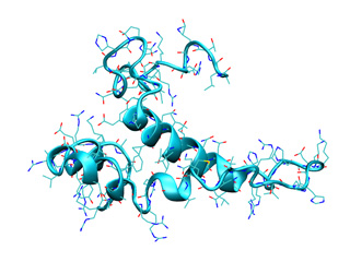
The iMOD Tutorial is a practical guide for researchers who want to perform NMA in Internal Coordinates to explore feasible conformations of protein and nucleic acids. We included four small tutorials with basic instructions for:
- iMODE Performing NMA in IC
- iMOVE Animating modes
- iMODVIEW Visualizing modes
- iMC Monte-Carlo in IC modal space
- iMORPH Morphing
We will use the structure of the ribosomal RNA binding protein S15 (1ab3, cyan) to illustrate a simple NMA calculation
In the Download section you can be found all the binaries and example files to complete the tutorial. Please, uncompress and untar the corresponding tutorial file. You will have all the necessary files to follow the tutoriales. We recommend to create a new working directory, so all the output files will be stored on it.
To compute the normal modes of a macromolecule, only the protein or nucleic acid structure is required in PDB format:
Please, ensure that input coordinates conform PDB format. The presence of all heavy atoms is mandatory; so be aware of missing atoms, alternative conformations, bad placed atoms and a long etc... that can eventually jeopardize your results. Use your favorite PDB checker to anticipate and fix any PDB error. We typically employ Molprobity (online), pdb2pqr (e.g. pdb2pqr file.pdb --ff=CHARMM ), profix from Jackal package or a combination of them.
Here is the screen output:
imode>
imode> Welcome to the NMA in Internal Coordinates tool v1.10
imode>
imode> Reading PDB file: 1ab3.pdb
molinf> Protein   1 chain  1   segment  1 residues: 88 atoms: 744
molinf> SUMMARY:
molinf> Number of Molecules ... 1
molinf> Number of Chain ....... 1
molinf> Number of Segments .... 1
molinf> Number of Groups ...... 88
molinf> Number of Atoms ....... 744
molinf>
imode> Coarse-Graining model: Full-Atom (no coarse-graining)
imode> Selected model residues: 88
imode> Selected model (pseudo)atoms: 744
imode> Number of Dihedral angles: 174
imode> Number of Inter-segment coords: 0 (Rot+Trans)
imode> Number of Internal Coordinates: 174 (Hessian rank)
imode> Range of computed modes: 1-20
imode> Creating pairwise interaction potential:
imode> Inverse Exponential (38974 nipas) cutoff= 10.0, k= 1.000000, x0= 3.8
imode> Packed-Hessian/Kinetic matrices mem.= 0.122 Mb (rank= 174)
imode> Fast Hessian Matrix Building O(n^2) 0.01 sec
imode> Fast Kinetic-Energy matrix Building O(n^2) 0.00 sec
imode> Eigenvector matrix mem. = 0.028 Mb
imode> Diagonalization with XSPGVX()... 0.25 sec
imode> Showing the first 10 eigenvalues:
imode>
imode> MODE   EIGENVALUE
imode>    1  4.88224e-04
imode>    2  8.38843e-04
imode>    3  1.45977e-03
imode>    4  1.94916e-03
imode>    5  2.10617e-03
imode>    6  3.41256e-03
imode>    7  3.54337e-03
imode>    8  4.74782e-03
imode>    9  5.23973e-03
imode>   10  6.38150e-03
imode>
imode>
imode> SAVED FILES:
imode> Log file:                                                      imode.log
imode> Model PDB:                                               imode_model.pdb
imode> ICS eigenvectors:                                          imode_ic.evec
imode>
imode> Bye!
By default, it saves the following files:
- imode.log --> Log-file.
- imode_model.pdb --> Used PDB model.
- imode_ic.evec --> Normal modes file.
With the normal modes files (eigenvectors and eigenvalues) you can either animate them to see how they look or perform a MC simulation. See next sections for details.
Once the modes were computed (iMODE), we are ready to see how is the motion that they describe. To animate the first mode (number 1) type at the command prompt:
Here is the screen output:
imove>
imove> Welcome to the Internal Coordinates Motion Tool  v1.07
imove>
imove> Input PDB-file imode_model.pdb
imove> Multi-PDB output file imove_1.pdb
imove> Number of frames to be generated 11
imove> Normal Mode choosen 1
imove> Reading PDB file imode_model.pdb
imove> Formatting residues names
imove> Coarse-Graining model: Full-Atom (no coarse-graining)
imove> Selected model number of residues: 88
imove> Selected model number of (pseudo)atoms: 744
imove> Ptraj info: imode_ic.evec  vectors=20  components=174
imove> Maximum internal coordinate displacement: 156.272797
imove> Dihedral coordinates found = 174
imove> Internal coordinates found (size) = 174
imove> Moving analiticaly (moving internal coordinates)
imove> Added frame    -5 to Multi-PDB
imove> Added frame    -4 to Multi-PDB
imove> Added frame    -3 to Multi-PDB
imove> Added frame    -2 to Multi-PDB
imove> Added frame    -1 to Multi-PDB
imove> Added frame     0 to Multi-PDB <-- 1st model (imode_model.pdb)
imove> Added frame     1 to Multi-PDB
imove> Added frame     2 to Multi-PDB
imove> Added frame     3 to Multi-PDB
imove> Added frame     4 to Multi-PDB
imove> Added frame     5 to Multi-PDB
imove>
imove> Success!
imove> Written movie: imove_1.pdb (11 frames)
imove> Bye!
The program output is a Multi-PDB file named: imove_1.pdb, with 11 MODELs. The motion is represented by equally spaced snapshots going from the negative end (MODEL -5) to the positive end (MODEL 5). The initial structure is the middle model (MODEL 0).
Below, you can see how the two lowest energy modes look like, either by clicking ![]() mode1 and
mode1 and ![]() mode2, or watching the corresponding flash movies.
mode2, or watching the corresponding flash movies.
By default, the amplitude (−a option) is set to twice its thermodynamic value predicted at room temperature (300K). Since true motion amplitude is unknown we encourage you to test different values in order to get the desired appearance. Also the number of modes is a interesting variable to investigate. In Lopez-Blanco et al. we found nice results with Cα and ED potential with default amplitude and number of modes. However, remember that iMC is a proof of concept sampling procedure and not ball-proof conformation ensemble generator, therefore you need to parametrize a bit the input variables. To this respect, any experimental evidence (Rg, distance constraints, etc. ) will be very helpful.
More modes can be observed clicking the following links: ![]() Mode3,
Mode3, ![]() Mode5,
Mode5, ![]() Mode10 and
Mode10 and ![]() Mode20.
Mode20.
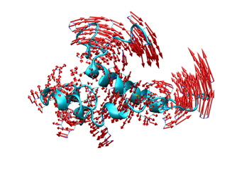
Any normal mode can be depicted as a 3D vector set. Each of them representing the relative atomic motion. The following command visualizes the first normal mode using red arrows. Note any VMD color can be used instead.
The unique output file 1ab3_1.vmd can be loaded into VMD using the following command in VMD's terminal:
vmd> source <out_vmd>
Since iMODVIEW only plots Cartesian normal modes, the use of --save_cart option in iMODE is mandatory. This way, an additional file with the Cartesian space modes will be generated: imode_cart.evec
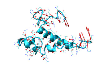
In addition, the averaged displacement vectors can be computed at several graining levels. To compute the average displacement over each atom (0), residue (1), segment (2) or chain (3), use the --level option followed by the corresponding number between brackets. Vectors will be located on the geometric center of averaged atoms. For example, the following command will compute the average displacement vectors over all residue atoms.
Below you can check previous commands results, for atomic and residue levels (left and right, respectively).
 |
 |
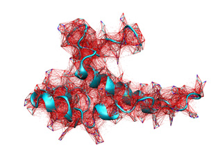
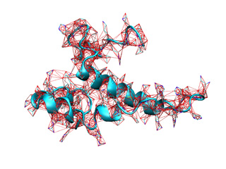
In addition, iMODVIEW can represent the spring network using straight segments. Their thickness will be proportional to their force constant (it can be adjusted using the --thick option).
This command will depict all available springs in force constants file. Also, you can adjust the range of plotted springs adding the --kthr and --kthr2 options to the basic command. For example:
In this case, only those springs with force constants above 0.5 will be represented. Results obtained from previous commands are shown below.
 |
 |
4) Monte-Carlo in IC modal space.
Once the modes are computed (iMODE) a MC trajectory can be obtained easily typing at the command prompt:
Here is the screen output:
imc>
imc> Mon's Monte-Carlo NMA-based trajectory program v1.07 (ADP-Platform)
imc>
imc> Reading Input PDB file
molinf> Protein   1 chain  1   segment  1 residues: 88 atoms: 744
molinf> SUMMARY:
molinf> Number of Molecules ... 1
molinf> Number of Chain ....... 1
molinf> Number of Segments .... 1
molinf> Number of Groups ...... 88
molinf> Number of Atoms ....... 744
molinf>
imc> Coarse-Graining model: Full-Atom (no coarse-graining)
imc> Selected model number of (pseudo)atoms: 744
imc> Opening output trajectory file: imc.pdb
imc> Dihedral coordinates found = 174
imc> Internal coordinates found (size) = 174
imc> Ptraj info: imode_ic.evec  vectors=20  components=174
imc> Number of used modes: 20
imc> ACEPTANCE RATIO(%): 40.319000
imc>
imc> Success!
imc> Written MC-trajectory: imc.pdb (100 frames)
imc> Bye!
The resulting Multi-PDB with the MC trajectory is: imc.pdb. The MC flash movie can be watched below; in addition you can see it in Jmol by following this link: ![]() MC trajectory.
MC trajectory.
5) Morphing in IC modal space.
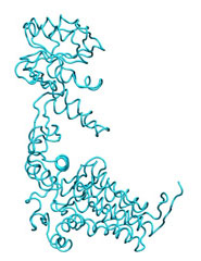
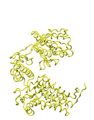
To illustrate the basic procedure and the method performance, we are going to morph the GroEL monomer in an open state (1aon, cyan) into the closed structure (1oel, yellow).
 |
M O R P H I N G open-->closed |
 |
The required input is minimal, just two protein or nucleic acid PDB structures with the same atoms. Input coordinates should conform to PDB format. Given the use of Internal Coordinates the presence of all heavy atoms is mandatory; so be aware of missing atoms, alternative conformations, bad placed atoms and a long etc... that can eventually jeopardize your results. Use your favorite PDB checker to anticipate and fix any PDB error. We typically employ Molprobity (online), pdb2pqr (e.g. pdb2pqr file.pdb --ff=CHARMM ), profix from Jackal package or a combination of them.
To perform the morphing just prompt:
Here is the screen output:
imorph>
imorph> Welcome to iMORPH v1.27
imorph>
imorph> Model PDB file: 1aon.pdb
molinf> Protein   1 chain  1   segment  1 residues: 524 atoms: 3847
molinf> SUMMARY:
molinf> Number of Molecules ... 1
molinf> Number of Chain ....... 1
molinf> Number of Segments .... 1
molinf> Number of Groups ...... 524
molinf> Number of Atoms ....... 3847
molinf>
imorph> Coarse-Graining model: Full-Atom (no coarse-graining)
imorph> Selected model number of residues: 524
imorph> Selected model number of (pseudo)atoms: 3847
imorph> Target PDB file: 1oel.pdb
imorph> Number of Inter-segment coords: 0 (Rot+Trans)
imorph> Number of Internal Coordinates: 1033 (Hessian rank)
imorph> Range of used modes: 1-206 (19.9%)
imorph> Number of excited/selected modes: 4(nex)
imorph>
imorph>  Iter      RMSD  RMSD(CA) NMA   NMA_time
imorph>     0 16.434504 16.013224   0       none
imorph>    53 15.610546 15.202492   1   3.74 sec
................................................
imorph>  1858  3.092514  2.640378  16   3.99 sec
imorph>  2631  2.268762  1.699723  17   4.60 sec
imorph> 10000  1.808299  1.151047            END
imorph>
imorph> Movie file:                            1aon_1oel_movie.pdb
imorph> Score file:                            1aon_1oel_score.txt
imorph> Log file:                                    1aon_1oel.log
imorph>
imorph> Success! Time elapsed 136.000
imorph> Bye!
By default, it saves the following files:
- imorph.log --> used command and parameters log
- imorph_score.txt --> score file to check for convergence
- imorph_movie.pdb --> morphing trajectory Multi-PDB
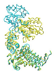
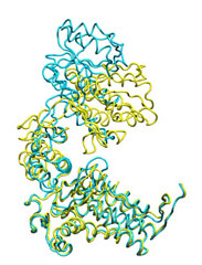
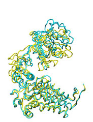
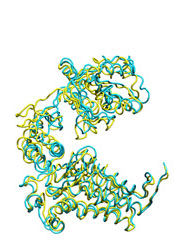
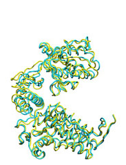
Below some morphing snapshots (cyan) are represented simultaneously with the target structure (yellow):
 |
 |
 |
 |
 |
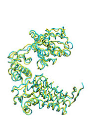 |
The morphing result is only 1.15Å Cα RMSD from the target. The quality of fitness and the excellent Secondary Structure maintenance can be appreciated in the flash movie below. Note that in none case any secondary structure constraint was used.
To analyze the trajectory ( imorph_movie.pdb ) we recomend VMD, but you are free to use your favorite program, as long as it reads Multi-PDB files. In addition you can observe the trajectory interactively: ![]() View in Jmol. The images and the movie were created with VMD using the POVray rendering engine.
View in Jmol. The images and the movie were created with VMD using the POVray rendering engine.
If not evident, it would be convenient to check out convergence. To this end just plot the RMSD as function of the iteration number using GNUplot:
> gnuplot -persist
> gnuplot> plot "imorph_score.txt" u 1:2 w l
> gnuplot> exit
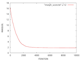 |
If the the slope is not approximately horizontal at 5000−10000 you can either run iMORPH again increasing the number of maximum iterations (−i), or alternatively you can continue the morphing process introducing the final structure as initial model. To this end, you should add previously the −−morepdbs option to force the final fitted structure output (imorph_fitted.pdb).
Note: The conformational refinement is an stochastic process; thus you should not expect to obtain exactly the same screen output and the same results between different runs.
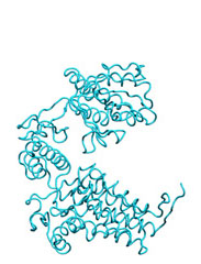
iMORPH allows to open "closed" structures as well. To perform this morphing just reverse the order of initial and target structures:
 |
M O R P H I N G closed-->open |
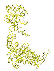 |
The initial closed structure, 1oel, is shown in cyan and target open structure, 1aon, in yellow. The −o option is added to avoid overwriting previous results.
The final structure is again very close to the target, i.e. 1.20Å Cα RMSD. As in above case, the quality of fitness and the excellent Secondary Structure maintenance are evident. Also, you can observe the trajectory interactively: ![]() View in Jmol.
View in Jmol.
