The inverse scattering problem
In principle the SAXS profile of any structure can be calculated at any resolution by approximating the structure by a set of closely packed spheres, whose SAXS profile can be calculated using the Debye formula (Debye, 1915). The procedure has been widely used in the past to derive the scattering profiles of many structures (Cantor and Schimmel, 1980), and CPU efficient algorithms exist now for speedy computation of the scattering profile of structures of even tens of thousands of scattering elements (Pantos et al. 1996). This work focuses on the inverse scattering problem, which consists of deducing the possible structure(s) or shape(s) or structural changes of a macromolecule, from its X-ray scattering profile to a given resolution. Contrary to the direct scattering calculation, the inverse problem can not be solved analytically, i.e., no "inverse Debye" formula can be constructed to yield 3D position coordinates from scattering data.
 At a first approximation the inverse scattering problem can be reduced to the search for a model compatible with the scattering profile in a pre-defined region of space discretized in finite particles (typically spheres). This procedure, consists of two steps: i) the computation of the scattering profile for each possible combination of these elements ii) the selection of the one which best fits the experimental profile. An exhaustive search approach using a CPU efficient computational method has been employed in a variant of program DALAI (Pantos and Bordas, 1994) to characterize the low resolution structures of tubulin microtubules (Andreu et al. 1992) and tubulin rings (Díaz et al. 1994) in solution. This method selects the best available configuration from a large set of candidates within a configurational space. This direct procedure is limited in scope because the exploration of all configurations becomes successively more difficult as the resolution, i.e., the number of spheres in a configurational space of given extent, increases beyond reasonable limits in computer memory and processing time. For example, the number of possible configurations in a space discretized into 79 elements is close to Avogadro's number (2e79 =6.044x10e23), a number too huge to be contemplated. Even if unsuitable configurations (e.g.,symmetry related ones or those with too few or too many spheres) are excluded from the computation of the Debye formula, those remaining to be examined are still too many, even to count, never mind processing them. In fact, the exhaustive search with built-in criteria for avoiding computation of unsuitable configurations (radius of gyration rejection test) using the parallel implementation of the DALAI code (Dean et al. 1994) has only been attempted with configuration spaces not exceeding 31 spheres in total (the 32-bit positive integer limit gives 231-1 = 2,147,483,647 possible configurations). This limit can only be exceeded by including a "hard-core" of spheres always present in the model and consequently not counting towards the number of configurations generated but allowing the use of models with larger volumes than that of 31 spheres. The number of iterations that can be performed to provide a sufficient level of confidence in the uniqueness of the solution is limited by practical considerations for the reasons explained above.
To overcome this problem it is necessary to apply an efficient search procedure. To this end, we have combined the Debye formula algorithm used in DALAI with an optimization tool: a genetic algorithm (GA). The result is a general method for deducing the possible low resolution structure of a macromolecule from its solution SAXS profiles. The method consists of fitting the scattering profile computed from sphere packet models of the molecule using the Debye formula. The models are optimized by means of a genetic algorithm that searches the huge space of possible mass distributions and evolves convergent models.
Andreu, J.M, J. Bordas, J.F. Díaz, J. García de Ancos, R. Gil, F.J. Medrano, E. Nogales, E. Pantos and E.Towns-Andrews. 1992. Low resolution structure of microtubules in solution. J. Mol. Biol. 226:169-184
Dean, C.E., R.C. Denny, P.C. Stephenson, G.J. Milne and E. Pantos. 1994. Computing with parallel vitual machines. J. Phys. III. Colloque C9:445-448.
Debye, P. 1915. Zerstreuung von röntgenstrahlen. Scattering from non-crystalline substances,Ann. Phys. 46:809-823.
Díaz, J.F., E. Pantos, J. Bordas and J.M. Andreu. 1994. Solution structure of GDP-tubulin double rings to 3nm resolution and comparison with microtubules. J. Mol. Biol.238:214-225.
Pantos, E. and J. Bordas. 1994. Supercomputer simulation of small angle x-ray scattering, electron micrographs and x-ray diffraction patterns of macromolecular structures. J.Pure and Appl. Chem. 66: 77-82.
Pantos, E., H.F. van Garderen, P.A.J. Hilbers, T.P.M. Beelen and van R.A. Santen. 1996. Simulation of small angle scattering from large assemblies of multi-type scatterer particles. J. Mol. Struct. 383:303-308.
Algorithm description
1) Mapping of the configuration space into a bit string.
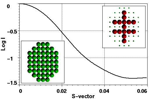
Figure 1a gives an example of a simple configurational space, a 7x9 regular grid of spheres masked by an ellipsoid, and the SAXS profile corresponding to one of the structures within it. The bit-string representation of this structure, the so-called chromosome, is
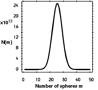
where the counting of bits (genes) is from left to right, top row to bottom row. Each one of the ON bits, corresponds to a unique coordinate position. The number of possible configurations is given by N(m)=n!(n-m)!/m! where n is the length of the chromosome and m is the bit-sum (the number of spheres in the structure). It is shown graphically in Figure 1b.
|
Figure 1. a) The SAXS profile of the structure shown in the top right insert within the configuration space of 51 spheres on a 7x9 grid with the corners of the rectangle masked off (bottom left insert). This structure can be found in 13 other symmetry equivalent positions. b) The number of configurations for mass in the range 1 to 51 spheres including symmetry related configurations.
Let us now consider the inverse problem: If the profile shown in Figure 2 is the "experimental data" how do we find the configuration that corresponds to it? An exhaustive search approach has been employed in a variant of program DALAI (Pantos unpublished ) to model the SAXS profile of the tubulin dimer used to build tubulin superstructures (Andreu et al. 1992, Diaz et al. 1994). This procedure is limited in scope because the exploration of all configurations becomes successively more difficult as the resolution, i.e., the number of spheres in a configurational space of given spatial extent, increases beyond reasonable limits. Searches have been made with configuration spaces not exceeding 31 spheres in total (231-1 =32-bit integer limit = 2,147,483,647 configurations). This limit can only be exceeded by including a "hard-core" of spheres always present in the model and consequently not counting towards the number of configurations generated but allowing the use of models with larger volume than that of just 31 spheres. The task becomes impossible for searches with no constraints on the minimum volume/shape and grid sizes commensurate with the resolution of the experimental data.
For example, the number of possible configurations in a space of 10x10x10 nm occupied by hard spheres of 1 nm radius, typical of grid sizes needed for proteins, is 21000-1, a number too huge to be contemplated even by cosmologists! To illustrate the point, the simple loop counting up to the Avogadro number (279=6.044x10²³)
count=count+1
ENDDO
would take some 200000 CPU years to execute on a MIPS-R1000 195 MHz processor.
Let us take the SAXS profile in Figure 1a as a simple test case and let us assume that we have some idea about the maximum extent of the target object (from the Rg value, electron microscopy or some other technique) represented by the extent of the configuration space. The number of possible configurations is now 251-1 = 2.25x10¹⁵. Each configuration corresponds to a potential solution for the mass distribution.
2) Generation of an initial population of chromosomes.
We now generate randomly a population of chromosomes each of them representing a different model structure within the configuration space. A set of 200 to 1000 is normally adequate in sampling the full mass range. Each chromosome is decoded into a set of coordinates by means of a look-up table containing all the possible (51 in this example) coordinates. The resulting structural models are processed by the SAXS simulation procedure to obtain the scattering profiles which are then compared with the experimental data by computing the fitness value defined as the normalized sum of residuals
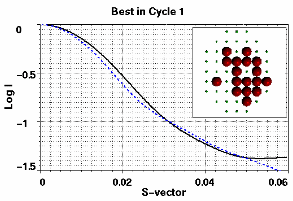
where n is the number of points in the profile and Icalc and Iexp the computed and experimental intensities, respectively, normalized at the first point. The profile of the best structure and the fitness values of the initial population are shown in Figure 2. It is obvious that the starting best guess structure is far from ideal.
3) Evolution of the breeding stock.
The algorithm now proceeds by selecting the elite portion of the current population (typically 10-30% of the total) which is used as the "breeding stock". Chromosomes are selected at random from this set and recombined by operators simulating genetic mechanisms: a) Uniform crossover takes two individuals, so-called parents, and mixes their genes randomly. b) Random mutation changes genes of offspring from 0 to 1 or from 1 to 0. The new set of offspring is processed by the SAXS simulation procedure after discarding accidental identical twins. A new ranking order is established and offspring that fit the target profile best are promoted into the breeding stock while unfit ancestors are discarded. This process is repeated in subsequent cycles. It is easy to see that the population will evolve over successive generations towards a global maximum.
 |
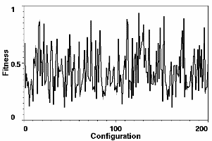 |
Figure 2. Left: The profile of the first best guess configuration (dashed line) compared with the target profile (solid line). Both profiles are normalized at the first point. The inset shows the first best guess structure of 17 spheres. Right: The fitness values of the starting guess structures. Their Rg and mass values span the range 7-27 and 4-36, respectively.
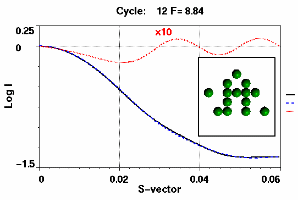
Figure 3 and Table I reflect the situation at an early stage in the evolution of the reproductive population. The algorithm has already generated top configurations with mass and Rg values not far from those of the target. The similarity with the target configuration is now beginning to emerge. This early success can be used to advantage by optionally narrowing down the mass range and Rg value of configurations needing to be processed by the SAXS simulation procedure in subsequent generations.
 |
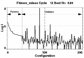 |
Figure 3. Left: Target profile (line) and current best fit (dashed line) produced at iteration 12. The dotted line shows the residual amplified x10. The current best structure is shown in the insert. Right: The fitness values of the current population. The top 30% make up the breeding stock ranked according to fitness. The rest are the new offspring, several of which will be promoted into the breeding stock in the next cycle. A new leader has been born with fitness value = 8.84. Configurations with zero fitness value are those which have been rejected on the basis of their mass or Rg value being outside a preset range.
| Table I. The 10 best configurations from generation 12. Columns 2 to 5 give the fitness value, the radius of gyration, the number of spheres and the configuration bit-string. | ||||
| 1 | 8.839 | 15.918 | 14 | 000 00100 0010100 1011110 0010100 0110101 0000000 00000 000 |
| 2 | 5.764 | 15.622 | 15 | 000 00100 0010110 1001110 0011101 0010100 0000100 00000 000 |
| 3 | 5.743 | 15.333 | 14 | 000 00000 0011110 0010101 0001101 0010101 0000010 00000 000 |
| 4 | 5.478 | 15.597 | 14 | 000 00100 0010100 1011110 0010101 0110100 0000000 00000 000 |
| 5 | 5.277 | 15.821 | 15 | 000 00100 0010110 1011110 0010101 0110100 0000000 00000 000 |
| 6 | 5.161 | 15.753 | 14 | 000 00100 0010110 1001100 0011101 0010100 0000100 00000 000 |
| 7 | 5.059 | 16.559 | 15 | 000 00000 0010111 1111100 0010101 0110100 0000000 00000 000 |
| 8 | 4.849 | 16.055 | 16 | 000 01010 0010100 0011110 0011101 0110100 0000000 00100 000 |
| 9 | 4.749 | 15.969 | 14 | 000 00100 0010100 1011110 0010100 0110100 0000000 00100 000 |
| 10 | 4.499 | 15.097 | 14 | 000 00000 0010100 0010111 0001101 0010101 0000110 00000 000 |
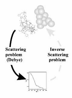
Figure 4 summarises the steps followed so far.
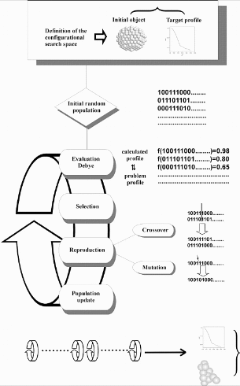
Figure 4. Schematic of the genetic algorithm implementation
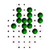
The graphs in Figure 5 are instructive on how convergence to the best fit is reached. In the early stages better candidates are produced rapidly. Improvements in the lead candidate occur at successively longer intervals as the breeding stock improves steadily (Darwinian selection pressure). It is this feature of the genetic algorithm that makes it so powerful. The procedure inevitably leads to the rebirth of chromosomes that have existed in a previous cycle, only to be discarded again. This apparent wastefulness of the algorithm is offset by the overall improvement achieved in the end. The total number of configurations required to be examined to reach the perfect fit for this example (Figure 6) was nearly 2x10⁶ (generated in 700 iterations), six orders of magnitude smaller than the number of configurations of mass 15, N(15)= 3.2x10¹² and 9 orders of magnitude smaller than the total number of configurations an exhaustive search would have had to process to be sure of finding the best fit. The lower graph in Figure 6 tells us that as time passes fewer and fewer offspring are likely to be better than their parents. The reason for this is that the number of "better" configurations that can be produced is decreasing rapidly, they are more difficult to find. At this point the system has converged and the search for better fits is driven mainly by the mutation process and accidental cross-breeding of configurations with appropriate sets of genes.
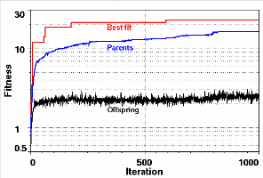
Figure 5. Semilog plots of the evolution of the best fit (upper curve), the average fitness value of the parents (middle curve) and the average fitness value of the offspring (lower curve). The quality of the breeding stock improves with iteration number.
 |
 |
 |
 |
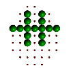 |
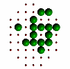
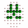
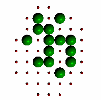
Figure 6. Evolution of successive best fit structures. The final structure is one of the 13 symmetry related ones to the target object in Figure 2a. Independent runs of the program (different starting seeds for the random number generator) may result to another solution (target shape in different orientation) at different times.
Cantor C.R. and P.R. Schimmel. 1980. Biophysical Chemistry. Part II. Techniques for the study of biological structure and function. W.H. Freeman, New York. 811-819.
