This tutorial is a practical guide for learn how to flexibly fit atomic models into low/medium resolution EM maps with IMODfit. We included some working examples with simple instructions, as well as a benchmark set. Before you go through the tutorial, first get the corresponding files from download zone. This tutorial is divided in three parts:
- Basic Flexible Fitting I. From open to close
- Basic Flexible Fitting II. From close to open
- The 52 proteins benchmark
Basic Flexible Fitting I. From open to close
First download, uncompress and untar the corresponding tutorial file. You will have all the necessary files to follow the tutorial. We recommend to create a new working directory, so all the output files will be stored on it.
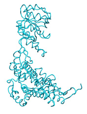
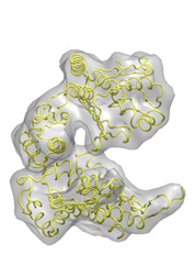
To illustrate the basic procedure and the method performance, we are going to fit the high resolution structure of GroEL monomer in an open state ( ![]() 1aon , cyan) into a 10Å resolution simulated EM closed map (grey) obtained from the closed structure (
1aon , cyan) into a 10Å resolution simulated EM closed map (grey) obtained from the closed structure ( ![]() 1oel , yellow).
1oel , yellow).
 |
F I T T I N G (open −−> closed) |
 |
To perform the fitting just type at the command prompt:
where 1aon.pdb is the initial structure, 1oel.ccp4 is the target map, 10 is the resolution in Angstroms, and 0 is the density cutoff to take into account map densities. The −t option enables the output of the PDB movie with the fitting trajectory. Here is the screen output:
imodfit>
imodfit> Welcome to iMODFIT v1.28
imodfit>
imodfit> Model PDB file: 1aon.pdb
molinf> Protein   1 chain  1   segment  1 residues: 524 atoms: 3847
molinf> SUMMARY:
molinf> Number of Molecules ... 1
molinf> Number of Chain ....... 1
molinf> Number of Segments .... 1
molinf> Number of Groups ...... 524
molinf> Number of Atoms ....... 3847
molinf>
imodfit> Coarse-Graining model: Full-Atom (no coarse-graining)
imodfit> Selected model number of residues: 524
imodfit> Selected model number of (pseudo)atoms: 3847
imodfit> Target Map file: 1oel.ccp4
imodfit> Best filtration method: 2 FT(x10)=0.090s Kernel(x10)=0.080s
imodfit> Number of Inter-segment coords: 0 (Rot+Trans)
imodfit> Number of Internal Coordinates: 1033 (Hessian rank)
imodfit> Range of used modes: 1-206 (19.9%)
imodfit> Number of excited/selected modes: 4(nex)
imodfit>
imodfit>  Iter     score     Corr. NMA   NMA_time
imodfit>     0  0.336409  0.663591   0   4.33 sec
imodfit>   157  0.319447  0.680553   1   4.52 sec
.................................................
imodfit>  4219  0.024751  0.975249  17   4.15 sec
imodfit> 10000  0.017593  0.982407            END
imodfit>
imodfit> Movie file:                              imodfit_movie.pdb
imodfit> Final Model:                            imodfit_fitted.pdb
imodfit> Score file:                              imodfit_score.txt
imodfit> Log file:                                      imodfit.log
imodfit>
imodfit> Success! Time elapsed  00h. 04' 04''
imodfit> Bye!
The flexibly fitted structure is: ![]() imodfit_fitted.pdb.
imodfit_fitted.pdb.
iMODFIT also outputs the following files:
- imodfit_movie.pdb --> fitting trajectory
- imodfit_score.txt --> score file to check for convergence
- imodfit.log--> used command log
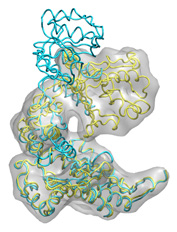
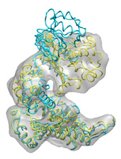
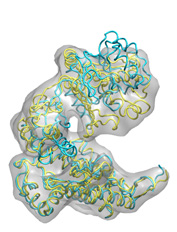
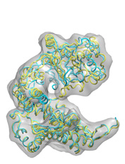
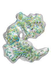
Below some fitting trajectory snapshots (cyan) are represented simultaneously with the target structure (yellow). The final snapshot with the fitted structure is shown on the right.
 |
 |
 |
 |
 |
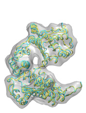 |
The fitting result is only 1.78Å Cα RMSD from the target structure, and the final correlation was high: 0.982. The quality of fitness and the excellent secondary structure maintenance can be appreciated in the flash movies below (front and rear views in left and right, respectively). Note that in none case any secondary structure constraint was used.
For visualizing the results use your favorite program. To play the trajectory movie ( imodfit_movie.pdb ) we recomend VMD; but you can see it in ![]() Jmol. The images and the movie were created using VMD with the POVray rendering engine.
Jmol. The images and the movie were created using VMD with the POVray rendering engine.
Once you have ran iMODFIT you should check for convergence. To this end just plot the score (i.e. 1−correlation) as function of the iteration number using GNUplot with the imodfit_score.txt file:
> gnuplot -persist
> gnuplot> plot "imodfit_score.txt" u 1:2 w l
> gnuplot> exit
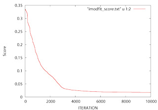 |
Note(1): If the the slope is not approximatelly horizontal at 5000−10000 you should run iMODFIT again to increase the number of maximum iterations (−i option). Alternatively you can continue the fitting process introducing the final fitted structure as initial model.
Note(2): The conformational refinement is an stocastic process; thus you should not expect to obtain exactly the same screen output and the same results between different runs.
Basic Flexible Fitting II. From close to open
iMODFIT allows to open "closed" structures as well. To perform this fitting just try the following command:
Front and rear views of the fitting results are shown in the flash movies below. The initial closed structure, 1oel, is shown in cyan, the target open one, 1aon, in yellow, and its corresponding open map in grey. The −o option is added to avoid overwriting previous results.
The final structure is again very close to the target, i.e. 1.74Å Cα RMSD (corr.=0.985). As in above case, the quality of fitness and the excellent Secondary Structure maintenance are evident. Also, you can observe the trajectory interactively: ![]() Jmol.
Jmol.
To test our methodology we build a benchmark formed by 52 simulated fitting problems, comprising a wide variety of macromolecular motions. To this end we downloaded from the molecular motions database MolMovDB 26 different protein pairs with displacements greater than 2Å Cα RMSD and sizes ranging from 100 to 1000 aminoacids. Only those structures with less than 3% Ramachandran outliers (Molprobity) and without broken chains and missing atoms were admitted. The average displacement was 6.9Å with a standard deviation of 3.9Å. Note that each open/closed protein pair represents two different fitting problems, i.e. from open to closed and vice versa. It can be downloaded either from the iMODFIT "Install" page or directly from here.
|
MolMovDB's Motion Types:
- Motions of Fragments Smaller than Domains
- [F-s-2] --> I.A. Motion is predominantly shear
- [F-h-2] --> I.B. Motion is predominantly hinge
- [F-?-2] --> I.C. Motion can not be fully classified at present
- [F-n-2] --> I.D. Motion is not hinge or shear
- Domain Motions
- [D-s-2] --> II.A. Motion is predominantly shear
- [D-h-2] --> II.B. Motion is predominantly hinge
- [D-?-2] --> II.C. Motion can not be fully classified at present
- [D-n-2] --> II.D. Motion is not hinge or shear
- [D-f-2] --> II.E. Motion involves partial refolding of tertiary structure
- Larger Movements than Domain Motions involving the Movement of Subunits
- [S-a-2] --> III.A. Motion involves an allosteric transition
- [S-n-2] --> III.B. Motion does not involves an allosteric transition
- [C----] --> C----. Complex Protein Motions