The Coarse Graining model representation determines both the system mass distribution and the springs network. The available Coarse-Graining models for proteins are listed below: Cα (−m 0) Only Cα atoms accounting for whole residue mase are considered.This CG model has two extra atoms per chain, one N atom at the begining and one C atom at the ending. 3BB2R (−m 1) There are five atoms per residue. Three representing the backbone: N, Cα and carbonylic C; and two representing the side chains: Cβ and a pseudo-atom (R) placed on the center of mass of the remaining side chain atoms. Note that Glycine and Alanine will be modeled by 3 and 4 atoms, respectively. Full-atom (−m 2, default) All heavy atoms are considered, each one accounting for its own mass. 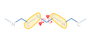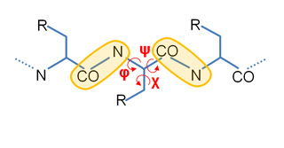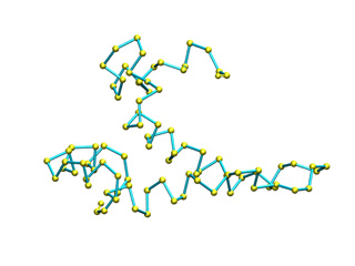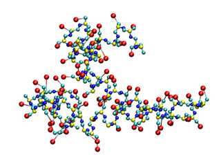Next figures illustrate the appearance of the Cα and 3BB2R CG models: Cα-model 3BB2R-model On the left model only Cα atoms (yellow) are considered. On the right, the 3BB2R model (right) have five atoms per residue: three representing the backbone (N, Cα and carbonylic C, in blue, yellow and cyan, respectively), and two representing the side chains (Cβ and a pseudo-atom placed on the center of mass of the remaining side chain, in cyan and red, respectively).  At this moment, only the Full-atom representation is available for nucleic acids: RNA DNA

To illustrate the usage of different CG models lets try the following examples:

• Computing modes at different CG levels.
• Monte-Carlo at different CG levels.
  

  --------------- Computing desired Normal Modes in different CG models. --------------- 

To choose the desired CG model -m option must be added to the basic command followed by model identifier. The basename option (-o) will be used to avoid overwriting of previous re.

You can check the CG models using Jmol:   Ca model and   3BB2R model.

In Ca case, an extra file is produced: imodeCA_ncac.pdb. This PDB file is just a standard PDB containing the coordinates of backbone nitrogen (N), and alpha (Ca) and carbonylic carbons (C), i.e. those atoms needed to define the f and ? dihedral angles. This is the minimum required structure to use our Ca model. A structure with only Ca atoms will not work. In this case, an external software to generate backbone N and C atoms is mandatory. For example, you can use the on-line server: SABBAC.

To animate this modes, the CG model introduced to iMOVE should be the same used in iMODE:

In Ca case there are less springs than in full-atom. Thus, the amplitude was lowered (-a 0.4). In 3BB2R case it is not neccessary such modification since the number of springs is similar to full-atom.

Its convenient to convert CG models to a full atom representation to avoid problems of compatibility with visualization software:

--------------- Monte-Carlo in different CG models. ---------------

To compute MC trajectories:

As before, to maintain the motion appearance the amplitude was lowered (-a 0.1) in Ca case.

To obtain full-atom trajectories from Ca or 3BB2R modes:

An extra output file named <basename>_icf.evec will contain the output modes of the corresponding CG level.

For a given structure and CG model, normal modes are determined by its potential energy, i.e. the spring network. In iMODE the potential energy can be customized several ways:

• By distance dependant functions.
• By topology and SS.
• User custom potential.

Distance dependant functions

Functions	Options*	Description
Inverse exponential (default) K = k/(1+(x/x0)^p), if x < c, else K=0	-P 0 --k0_c 10 --k0_k 1 --k0_x0 3.8 --k0_p 6	Distance cutoff (Å) Scale factor Inverse exponential center Power term
Simple distance cutoff K = k, if x < c, else K=0	-P 1 --k1_c 10 --k1_k 1	Distance cutoff (Å) Scale factor

*Bold options are mandatory.

For example, to use a Ca model with potential energy based on distance dependant functions, type:

The appearance of this potential energy models with default parameters is shown below. Springs are represented by red segments with thickness proportional to the force constant.

Inverse exponential (Stiffness inversely proportional to distance)	Simple distance cutoff (Constant stiffness)

To customize the potential energy funcitons modify the default options; for example:

Topology and Secondary Structure

iMODE permits the specification of customized inverse exponential functions according to both topology and SS.

The basic command for topology and SS would be:

A functions file (funcTSS.txt) is mandatory. It should conform the following format:
(Note, "#"-begining lines will be omitted)

# SS  n  k  x0 p
HH    0  2 3.8 6
HH    1  5 3.8 6
HH    2  3 3.8 6
HH   -1  2 3.8 6
EE    0  2 3.8 6
EE    1  5 3.8 6
EE    2  3 3.8 6
EE   -1  5 3.8 6
XX   -1  1 3.8 6

Each line represents an inverse exponential function. First column specifies the SS. For example, "HH" indicates that both atoms should belong to residues with a-helix SS. By default SS identifiers are: "H" helix, "E" strand, and "C" coil; and any pair of them is allowed. Second column specifies the topology. Here topology represents the sequential distance between two residues; for example, if our protein sequence were ...AGKTLV..., the topology between underlined residues would be 3. Remaining columns define the inverse exponential functional parameters: k, x0 and p, (see the table above).

The wildcards for SS and topology are "XX" and "-1", respectively.

By default, the SS is computed internally, but any user defined SS can be provided using the --ss option:

For example, you can use DSSP to compute SS (1ab3.dssp) and with the aid of this simple perl script you can convert it into our SS file format (1ab3.ss)

Our SS file format (1ab3.ss) is a simple two column ASCII file. The first column corresponds to the sequence index, and the second one to a single character SS identifiers.  

Customize potential energy by topology only.

The basic command for topology is:

The topology functions file (funcTOP.txt) is:

# SS  n  k  x0 p
XX    0  2 3.8 6
XX    1  9 3.8 6
XX    2  5 3.8 6
XX    3  3 3.8 6
XX    4  2 3.8 6
XX   -1  1 3.8 6

Customize potential energy by SS only.

The command to take into account SS only would look like this way:

The functions file (funcHE.txt) is:

# SS (j-i) k  x0 p
HH     -1  2 3.8 6
EE     -1  5 3.8 6
HE     -1  3 3.8 6
XX     -1  1 3.8 6

This file applies different functions to atom pairs belonging to residues with SS: H vs. H (HH), E vs. E (EE) and H vs. E (HE). The XX function will be applied to remaining pairs of atoms.

Given the non-Helical or non-Sheet regions are more flexible than the rest, some times may be interesting to increase flexibility in those regions. Corresponding command would be:

The functions file (funcCX.txt) is:

# SS (j-i)   k  x0 p
CC     -1  0.2 3.8 6
XX     -1    1 3.8 6

The springs associated to last example are represented below. First and second function springs are colored in orange and red, respectively. For clarity bo th kinds of springs were shown with similar thickness.

--------------- User custom potential. ---------------

The user can define its own potential thought a file using the -K option. Type at the command prompt:

This ASCII file (imodeKi_Kfile.dat) has three columns to define the force constants (K) for each atomic pair:

1 2 9.962940E-01
1 3 9.292819E-01
1 4 6.086772E-01
1 5 9.329874E-01
1 6 8.701856E-01
...........

Each line represents one spring. The first and second colums are the atomic indices (begining with 1), and the third is the force constant.

To obtain a Kfile template for your macromolecule that you can adapt to your convenience, use:

The resulting file, imodeKc_Kfile.dat, will contain the force constants for current potential energy model, in this case, the simple cutoff model.

In iMOD, the maximum macromolecular size allowed to perform NMA is constrained by the amount of memory needed to diagonalize the Hessian matrix, and it depends on the employed architecture. For example, in a standard 32-bit linux box (the maximum memory addressed per program is about 2Gb) so it can solve systems up to approximately 15000 degrees of freedom (DoF), i.e. about 7000-8000 aminoacids in proteins or 3000 nucleotids in nucleic acids. On the other hand, 64-bit machines are only limited by available RAM. For example, NMA of a 50000 DoFs system would need a 64-bit computer with about 30Gb of RAM memory. Therefore  a dimensionality reduction is mandatory when the system under study becomes huge for standard computers. To this end, we can fix some internal coordinates (ICs)  to reduce the number of degrees of freedom and fit the matrices into memory. There are three ways to accomplish this:

• Fixing custom ICs.
• Fixing by secondary structure
• Fixing ICs randomly.

Here we are going to comment the simplest way to reduce the dimensionality, which is to fix randomly some ratio of dihedral angles. Other possibilites to fix IC will be discussed in the next section.  Fixing ICs randomly For fixing randomly some ratio of dihedral angles, just type: This will fix the 50% of available dihedral angles. Note the inter-chain rotational/translational degrees of freedom are always maintained mobile. To illustrate this reductionist approach we purpose the following practical examples with a HUGE viral system:

• NMA of the closed CCMV capsid
• Morphing the closed CCMV capsid into the swollen form

NMA of the closed CCMV capsid

---

The capsid of the Cowpea Chlorotic Mottle Virus (CCMV) is a huge protein structure composed of 180 chains, 28620 aminoacids and 214440 atoms. In terms of ICs it means about 58000 ICs: 56994 dihedral angles (f and ?) and 1074 inter-chain rotational/translational variables. Perform NMA with 58000 ICs it's impractical in  standard PC box, since there would be needed a 64-bit computer with about 30Gb of RAM memory, and each diagonalization step would last even days. To overcome this we are going to fix the 90% of dihedral angles while keeping mobile all rotational/traslational degrees of freedom:

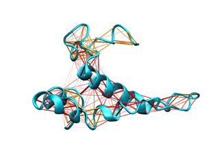
imode>
imode> Welcome to the NMA in Internal Coordinates tool v1.10
imode>
imode> Reading PDB file: 1cwp_prot.pdb
molinf> Protein   1 chain  1 A segment  1 residues: 149 atoms: 1122
molinf>                    2 B segment  1 residues: 164 atoms: 1226
molinf>                    3 C segment  1 residues: 164 atoms: 1226
molinf> Protein   2 chain  1 A segment  1 residues: 149 atoms: 1122
...................................................................
molinf> Protein  60 chain  1 A segment  1 residues: 149 atoms: 1122
molinf>                    2 B segment  1 residues: 164 atoms: 1226
molinf>                    3 C segment  1 residues: 164 atoms: 1226
molinf> SUMMARY:
molinf> Number of Molecules ... 60
molinf> Number of Chain ....... 180
molinf> Number of Segments .... 180
molinf> Number of Groups ...... 28620
molinf> Number of Atoms ....... 214440
molinf>
imode> Coarse-Graining model: Full-Atom (no coarse-graining)
imode> Selected model residues: 28620
imode> Selected model (pseudo)atoms: 214440
imode> Number of Dihedral angles: 55920
imode> Number of Inter-segment coords: 1074 (Rot+Trans)
imode> Number of Internal Coordinates: 56994 (Hessian rank)
imode> Input CG-model Fixed Internal Coordinates: 50328
imode> Input CG-model Final Internal Coordinates (sizei) = 6666
imode> Range of computed modes: 1-20
imode> Creating pairwise interaction potential:
imode> Inverse Exponential (16245240 nipas) cutoff= 10.0, k= 1.000000, x0= 3.8
imode> Packed-Hessian/Kinetic matrices mem.= 177.769 Mb (rank= 6666)
imode> Fast Hessian Matrix Building O(n^2) [hessianMFAx()] 17.24 sec
imode> Fast Kinetic-Energy matrix Building O(n^2) [kineticMFAx()] 20.34 sec
imode> Eigenvector matrix mem. = 1.067 Mb
imode> Diagonalization with XSPGVX()... 380.06 sec
imode> Showing the first 10 eigenvalues:
imode>
imode> MODE   EIGENVALUE
imode>    1  1.72062e-04
imode>    2  1.75517e-04
imode>    3  1.77022e-04
imode>    4  1.79158e-04
imode>    5  1.81447e-04
imode>    6  3.30420e-04
imode>    7  3.39147e-04
imode>    8  3.44462e-04
imode>    9  3.57581e-04
imode>   10  3.65270e-04
imode>
imode>
imode> SAVED FILES:
imode> Log file:                                                   1cwpDH09.log
imode> Model PDB:                                            1cwpDH09_model.pdb
imode> Fixation mask file:                                         1cwpDH09.fix
imode> ICS eigenvectors:                                       1cwpDH09_ic.evec
imode>
imode> Bye!

This way, only 6666 ICs were considered. Below you can check 5th and 18th normal modes, from the H and A and irreducible representations, respectively. On the left, the flash movies, on the left the displacement vectors.

Morphing the Closed CCMV capsid into the swollen form To illustrate iMORPH's performance on a huge system we are going to compute a feasible trajectory from the closed into the swollen structure. This "swelling", represents a huge concerted motion about 24.0 Å Ca RMSD where 2nm sized openings appear in the protein shell. Both structures were obtained from V IPERdb and are shown below. As a consequence of both motion and system size we had to carry it out in two steps using some extra options: imorph 1cwp_prot.pdb ccmv_swln_1_full.vdb -i 200000 -r 1 -e 0.05 --morepdbs --nowrmsd -o ccmvmorph
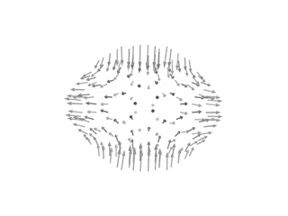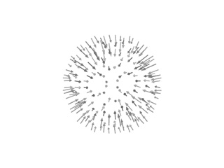imorph ccmvmorph_fitted.pdb ccmv_swln_1_full.vdb -i 300000 -r 1 -n 0.99999 --morepdbs --prob plain -o ccmvmorph2 In first step we added: -e 0.05 to speed up convergence, --nowrmsd to disable the Weighted-RMSD alingment (which is not suited to huge motions), and --more_pdbs to force saving the fitted structure. Note this fitted structure was still about 5 Å Ca RMSD away form target. In a second refinement step, we used all available modes (-n 0.99999) with a different mode selection scheme (--prob plain). Since we were closer to the target structure, the --nowrmsd option was removed. Note that to minimize NMA time in both steps only the rotational/translational ICs were considered (-r 1). Now a successful morphing result is obtained. It's only 0.95 Å Ca RMSD from target structure. You can check its beautiful movie below.

With iMOD you can fix in many ways the internal coordinate variables to reduce dimensionality of the problem:

• Randomly (commented before Q4) 
• Un-fix χ dihedral angle.
• By Secondary Structure.
• Customized  IC subset.

Un-fix any χ dihedral angle

---

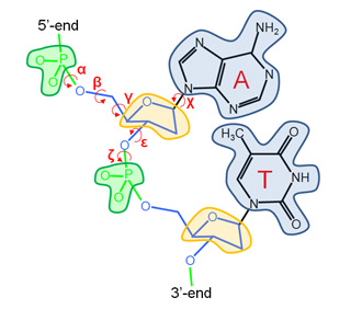
Our Internal Coordinates are: φ, ψ and χ dihedral angles for proteins, and α, β, γ, ε, ζ and χ for nucleic acids (see figure below). Another six additional rotational/traslational degrees of freedom are added every extra chain

Protein	RNA

By default we consider all but χ. The removal of this angles does not affect the low energy modes and will reduce the problem dimensionality around 1/2 in proteins and 1/5 in nucleic acids.

By secondary structure

---

With iMOd tou can fix the ICs depending on the secondary structure SS it belongs to. This can be done using the −−ss option followed by a letter identifiyer (H for helix, E for beta strands and C for others). Note you may fix any combination of SS by adding an identifier as you need; for example, "−S EC" will fix beta and coil. To fix all ICs related to α-helices and β-sheets, just type prompt:

By default, the SS is computed internally, but any user can defined it own SS throught a file and using the −−ss option:

For example, you can use DSSP to compute SS (1ab3.dssp) and with the aid of this simple perl script you can convert it into our SS file format (1ab3.ss)

Our SS file format (1ab3.ss) is a simple two column ASCII file. The first column corresponds to the sequence index, and the second one to a single character SS identifiers.  

Fixing custom ICs

---

Finally, you can fix any domain/s or region/s of your macromolecular structure. Any IC set can be considered fixed using the −f option with a mask file as;

where the mask file imodeFIX.fix is an ASCII file with four columns. The first column is the residue index (begining with 0), and the rest represents the φ, ψ and χ dihedral angles, respectively. In nucleic acid case, the file will have seven columns instead of four,  to account for the (six) α, β, γ, ε, ζ and χ dihedral angles.

A dummy mask (fully mobile) can be obtained using the −−save_fixfile option in iMODE program.

such mask looks like:

0 0 0 1
1 1 0 1
.........
276 1 0 1
277 0 0 1
278 1 0 1
.........
522 1 0 1
523 0 0 1

To customize just change "1" by "0" for fixing ICs, save it, and use with imode with −f option to load it and restric the NMA only with the non-fixed ICs as variables.

The extra zeros at some lines account for residues lacking corresponding ICs, i.e. Glycines and Alanines (no χ), and Prolines (no φ and χ). Note that the −x option must be added on previous commands if you plan to keep mobile some χ dihedral angles. If the macromolecule had several chains, six inter-chain rotational/traslational ICs are added: three x, y and z traslations and three rotations around x, y and z axis, respectively. For example, if there is a new chain after residue 187 (index 186) the mask file will be:

.........
186 1 0 1
187 1
187 1
187 1
187 1
187 1
187 1
187 1 0 1
.........

Any domain/s in our macromolecule can be fixed using the −f option. This way both dimensionality will be reduced and undesired distortions will be avoided. For illustrative purposes we will fix two GroEL domains.

GroEL is composed of three domains: apical (top red), intermediate (cyan), and equatorial (bottom red). The apical domain interacts with folding intermediates and GroES, the equatorial domain hydrolyzes ATP, and the intermediate domain is flexible and connects these apical and equatorial domains.

To obtain a successful fitting the structure should be maintained as flexibile as possible, i.e. if we fix very much the structure will be very rigid and the target conformation will not be addressed. To this end the apical and equatorial domains will be fixed while keeping the intermediate domain fully flexible. In the mask file imodfitDOM.fix only the ICs belonging to regions of the intermediate domain are keept mobile: 136-193 and 331-409 (indexed from 1 to 524). Further information about the mask file generation is provided in Q1 within this FAQ.

The output is the following:

imodfit>
imodfit> Welcome to iMODFIT v1.28
imodfit>
imodfit> Model PDB file: 1aon.pdb
molinf> Protein 1 chain 1 segment 1 residues: 524 atoms: 3847
molinf> SUMMARY:
molinf> Number of Molecules ... 1
molinf> Number of Chain ....... 1
molinf> Number of Segments .... 1
molinf> Number of Groups ...... 524
molinf> Number of Atoms ....... 3847
molinf>
imodfit> Coarse-Graining model: Full-Atom (no coarse-graining)
imodfit> Selected model number of residues: 524
imodfit> Selected model number of (pseudo)atoms: 3847
imodfit> Target Map file: 1oel.ccp4
imodfit> Best filtration method: 2 FT(x10)=0.090s Kernel(x10)=0.080s
imodfit> Number of Inter-segment coords: 0 (Rot+Trans)
imodfit> Number of Internal Coordinates: 1033 (Hessian rank)
imodfit> Input CG-model Fixed Internal Coordinates: 760
imodfit> Input CG-model Mobile Internal Coordinates (size) = 273
imodfit> Range of used modes: 1-54 (19.8%)
imodfit> Number of excited/selected modes: 1(nex)
imodfit>
imodfit> Iter score Corr. NMA NMA_time
imodfit> 0 0.336409 0.663591 0 0.73 sec
imodfit> 199 0.324457 0.675543 1 0.50 sec
imodfit> 379 0.285427 0.714573 2 0.49 sec
.................................................
imodfit> 12857 0.080700 0.919300 14 0.50 sec
imodfit> 50000 0.064124 0.935876 END
imodfit>
imodfit> Movie file: imodfitDOM_movie.pdb
imodfit> Final Model: imodfitDOM_fitted.pdb
imodfit> Score file: imodfitDOM_score.txt
imodfit> Log file: imodfitDOM.log
imodfit>
imodfit> Success! Time elapsed 00h. 16' 18''
imodfit> Bye!

The solution is only 3.77 Å Cα RMSD from the target structure used to simulate the map. This is a good result for a structure with 75% of its ICs fixed. Note that, to obtain a good result with such a fixed structure, the number of iterations was increased (-i 50000). If you increase the number of iterations even more you will reach lower RMSD.

You can play interactively the trajectory movie in Jmol, check the fitted structure imodfitDOM_fitted.pdb and watch the flash movie below. For illustrative purposes the fixed domains were colored in red.